Signal Vizualizers
Animated visualizers for signal processing.
Pages
Home
Signals
Fourier
Convolution
Filters
Developed by
Tom Donoghue.
Filters
This section explores applying (FIR) filters to time series.
Filters as Convolution
Applying a filter to a time series can be visualized as the convolution of a filter kernel with the data.
First, we can use a simplified example showing the application of a filter kernel (for a narrowband bandpass filter) to a burst signal:

Next, we can look at a applying a filter kernel to a ‘combined’ signal:

Applying a filter does not guarantee the extraction of a rhythmic component of the signal.
For example, we can see this in the ‘ringing’ in the output of applying a filter to a step function:

Notably, due to the shape of the filter kernel, outputs will tend to be smooth & rhythmic, even if the original data is neither.
For example, if we apply a bandpass filter to aperiodic (pink noise) data (non-rhythmic by definition) - the filter output still looks rhythmic:

Filter Outputs
Another way to look at filter outputs is to compare the outputs across different filter kernels.
First, we can see how the output varies across different n_cycles, when applied to a burst signal:

Next, we can see how the output varies across different bandwidths:

We can do the same for a step function signal, first with n_cycles:

And also with bandwidths:

Filter Properties
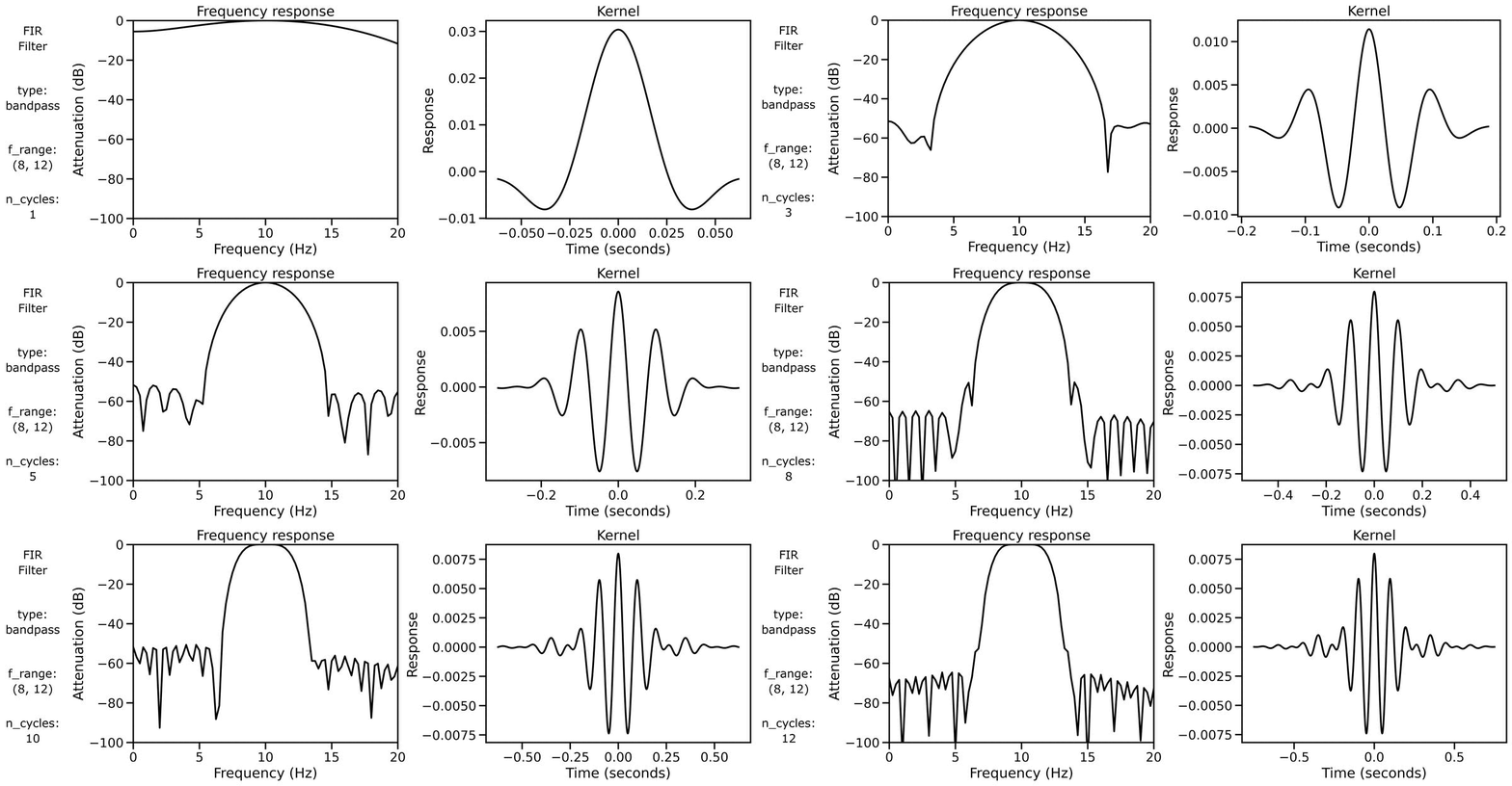
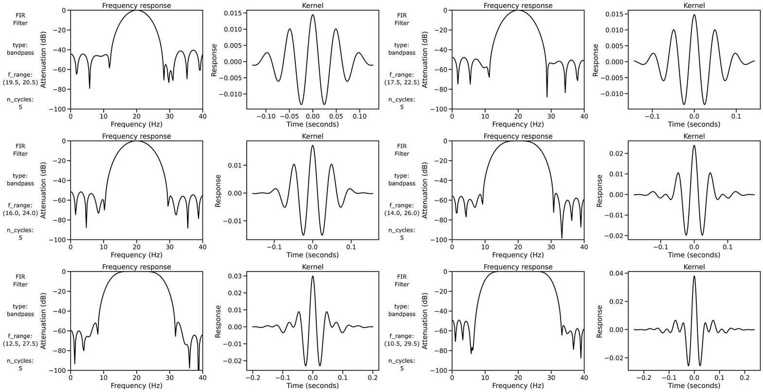
Finally, we can examine filter properties, explicitly examining the frequency response and filter kernel across different filter definitions.
First, we can look at the filter properties applied to a burst signal across different n_cycles:

We can also look at the filter properties applied to a burst signal across different bandwidths:
